In a previous case study, we explored how deep learning can be employed to automatically segment defects — an essential first step toward accurate quality control.
In this case, we focus on the next step: quantitatively measuring and classifying these defects. We discuss common standard tools available in most software packages and delve deeper into developing highly specific inspections through scripting. Whether such custom solutions are necessary depends on the specifications of the component being analyzed.
Standard porosity metrics
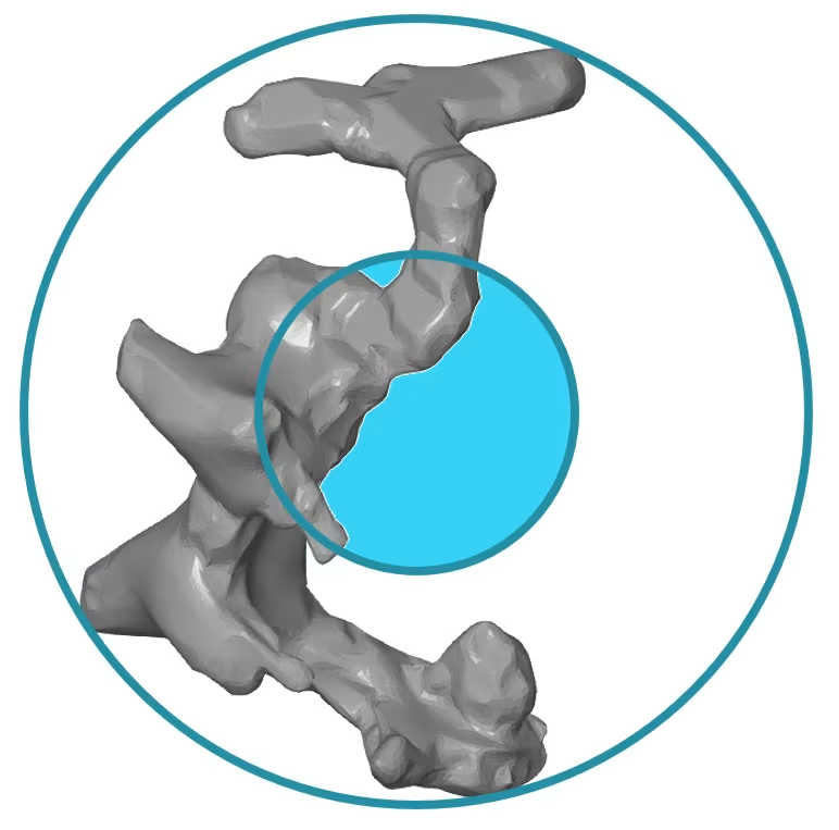
On the right-hand side, an example is shown of a defect that was segmented from a very high-resolution CT scan. To accurately characterize this defect, the software provides various standard metrics.
- Volume – e.g. 0,0003496 mm³
- This speaks for itself and shows the volume of each individual defect. The drawback is that these usually involve very small values, which can be more difficult to interpret.
- Equivalent Diameter – e.g. 0,087 mm
- This shows the diameter of a sphere with the same volume as the defect, and this number is somewhat easier to visualize.
- Defect Diameter
- The smallest possible or enclosing sphere that fully contains the defect.
- Compactness
- This shows the ratio of the defect’s volume to the volume of the enclosing sphere.
- Sphericity
- This shows the ratio of the surface area of the defect to the surface area of a sphere with the same volume.
Visualization of defect properties
Each individual defect can be characterized using one or more of the available standard measurements. Most software packages also offer the ability to visually display this data in the form of a color plot. In such a plot, each defect is assigned a color based on its specific value within a selected metric, such as volume or sphericity. This makes it easy to identify trends, anomalies, or critical areas at a glance.

The same data can also be presented in graphical form.

Overview of all defects
In a typical inspection report, we usually provide a clear summary of the detected defects. In the case of this manifold, a total of 29.070 defects were found, of which 116 are larger than 0.1 mm according to the specifications. In the two views below, only these larger defects are visualized, allowing you to quickly see exactly where they are located.

Advanced measurements on defects
For this specific manifold, it is not sufficient to rely solely on the standard defect measurements. According to the product specifications, additional parameters must be checked to ensure that the minimum wall thickness requirements are met.
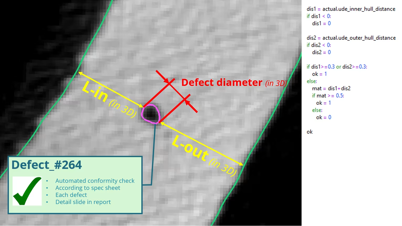
Therefore, in addition to the already available defect diameter, two additional distances are calculated:
- The smallest 3D distance between the defect and the inner wall of the manifold
- The smallest 3D distance to the outer wall
Based on this data, rules can be applied to automatically evaluate whether the material surrounding the defect still provides sufficient structural integrity. This type of customized inspection typically requires additional scripts or tailored workflows within the analysis environment.
Further reporting of all defects
Since we now have all possible measurements for each defect available, we can also automatically generate certain report pages. Below is an example of a detailed page for a defect that was found to be non-compliant according to the specifications.

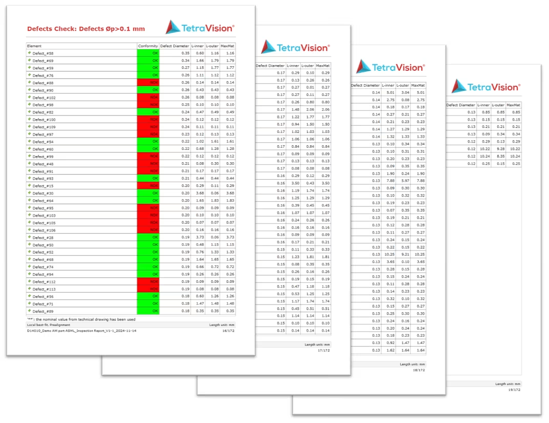
The results of all 116 defects can also be easily compiled into a summary table.
Additional wall thickness measurements
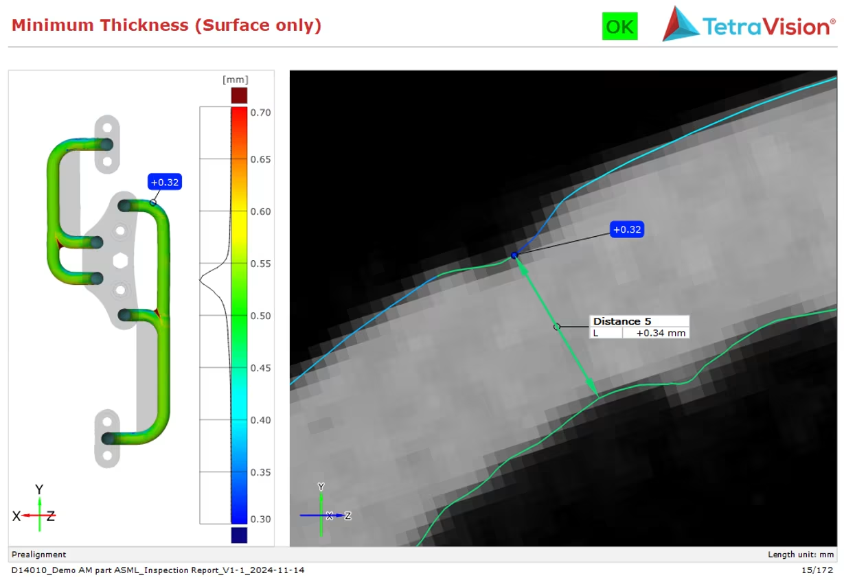
For the areas where no defects are present, it is still important to check the wall thickness. To do this, a standard wall thickness plot is generated between the inner and outer walls of the manifold. The minimum thickness is automatically detected, and a detailed image of this area is also added to the report.
Dross or excess material
Finally, we also automatically identify the areas with the largest dross. These are very localized zones of excess material. The risk is that this material could detach during the use of the manifold and potentially cause problems elsewhere in the machine. According to the specifications, this dross must therefore not exceed a certain size.
To do this, we generate a type of roughness plot that maps the local peaks and valleys of the inner wall. The largest values can then be automatically identified and included in the inspection report.

A report page with a detailed image based on the CT data of that same zone looks like this: